Introduction to Pandas

pandas is a Python library that makes it easy to read, export and work with relational data. This lesson will expand on its functionality and usage.

Use pip install pandas==0.24.2 to install the same version that we are using.

We typically import pandas as pd to refer to the library using the abbreviated form.

Pandas Series

From the official documentation, a Series is a one-dimensional ndarray with axis labels. A ndarray is a special data type found in the numpy library which defines an array of fixed size elements. In simpler terms, a Series is a column in a table or spreadsheet with the same data type. Each Series has an index used to indicate the axis labels.

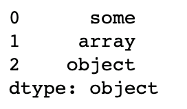
We can create a Series using pd.Series(['some', 'array', 'object'])

Indexing Series

We can look up Series values using the axis labels or by their positional labels. If not specified, the Series axis labels (otherwise known as the Series index) will default to integers. We can set the index to strings too.

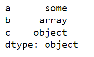
sample_series = pd.Series(['some', 'array', 'object'], index=list('abc'))
 
# positional indexing: this returns the first value, which is 'some'
sample_series[0]

# label indexing: this also returns the first value 'some'
sample_series['a']

This is what our sample_series looks like.

We can slice a Series to grab a range of values. Slicing behavior is different when using the axis labels -- contrary to usual Python slices, both the start and the endpoint are included!

# positional slicing: this returns the first two values
sample_series[:2]

# label slicing: this also returns the first two values
sample_series[:'b']

Pandas DataFrames

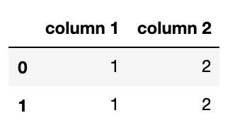
DataFrames are used to define two-dimensional data. Rows are labelled using indices and columns are labelled using column headers. Each column can be interpreted as a Series. We can create a DataFrame using pd.DataFrame({'column 1': [1, 1], 'column 2': [2, 2]}).

Alternatively, we can also read tabular data into DataFrames.

# Read in a CSV file
csv_dataframe = pd.read_csv('my_csv_file.csv')
 
# Read in an Excel file
xls_dataframe = pd.read_excel('my_xls_file.xls')

Indexing DataFrames

We can index DataFrame columns using square brackets. Let's use the very simple DataFrame we created as an example.

sample_dataframe = pd.DataFrame({'column 1': [1, 1], 'column 2': [2, 2]})
 
# get the column 'column 1'
sample_dataframe['column 1']

For more complex indexing, we can use .iloc or .loc.

Because we did not specify the axis labels for the rows, they adopted the default integer values. As such, the positional labels and axis labels are the same for this DataFrame.

We can retrieve the first row like this:

sample_dataframe.iloc[0, :]

sample_dataframe.loc[0, :]

Try it yourself!

Exploring a Synthetic Dataset with Pandas

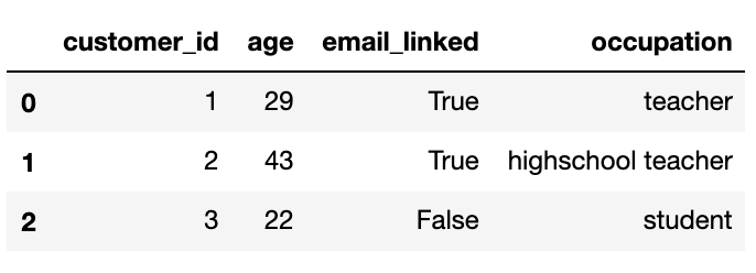
Let's create another DataFrame to illustrate some of the functionalities. We can pretend that this data is taken from a company that distributes education materials.

data = pd.DataFrame({'customer_id': [1,2,3,4,5,6,7,8], 
                     'age': [29,43,22,82,41,33,63,57], 
                     'email_linked': [True,True,False,True,False,False,True,True],
                     'occupation': ['teacher','highschool teacher','student','retired',
                                    'tutor','unemployed','entrepreneur','professor']})

For larger DataFrames, we can use.head(n) to look at the first n rows. To see the last few rows, we can perform a similar operation using .tail(n). Neither are necessary for our small dataset, but we can still demonstrate using data.head(3).

Filtering and Indexing a DataFrame

Assume that we want to run an email campaign. We start by extracting relevant columns to conduct our campaign.

# use double brackets to index multiple columns, single brackets for one column
email_data = data[['customer_id', 'email_linked']]

Not all of our customers have emails, so we definitely want to exclude those that don't.

# the condition goes inside the square brackets
email_data = email_data[email_data['email_linked']]

Applying a Column-wise Function

Let's write a very simple function to determine if a customer is an educator. This is how we define educator.

def is_educator(occupation):
    return 'teacher' in occupation.lower() or occupation.lower() in ['tutor', 'professor', 'lecturer']

We can apply this function onto the occupation column to create a new column.

data['is_educator'] = data['occupation'].apply(is_educator)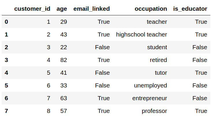

We can also transform all the rows in each column of a DataFrame. This requires that we set axis=0 (which is also the default setting). We can write a column-wise function to remove any columns that contain missing values. This is for demonstration only -- there are better ways to handle missing values (see the official pandas documentation for more detail)

def remove_missing_columns(col):
    if col.isnull().values.any():
        return col

data.apply(remove_missing_columns, axis=0)

Applying a Row-wise Function

We can also apply a function to transform every column in a row. This requires that we set axis=1.

def is_educator_above_50(row):
    return row['age'] > 50 and is_educator(row['occupation'])

data['is_educator_above_50'] = data.apply(is_educator_above_50, axis=1)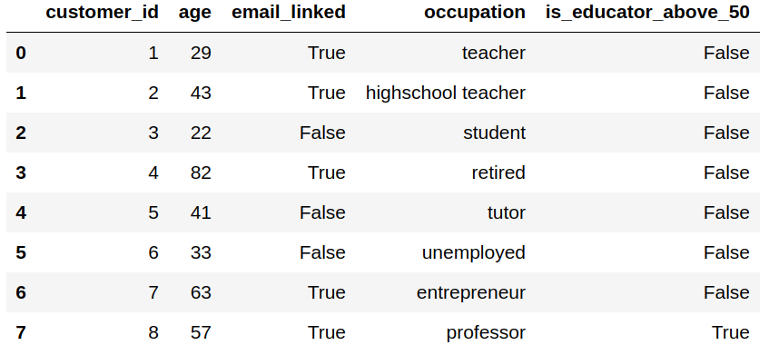

Groupby Operation

Groupby operations are useful for analyzing Pandas objects and engineering new features from large amounts of data. All groupby operations can be broken down into the following steps:

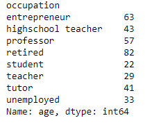
Typically, the object is split based on some criteria, a summary statistic is calculated for each group and combined into a larger object. We can use a groupby operation to calculate the average age for each occupation.

The code for this operation is very simple: data.groupby(by=['occupation']).mean()['age']

The by parameter indicates how groups are determined, mean() is the statistic of interest and indexing by age grabs the group statistic for age. The output is a series where occupation are the axis labels.

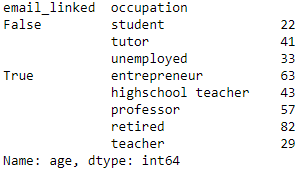
We can split groups using multiple parameters, for instance a combination of occupation and whether or not their email is linked: data.groupby(by=['email_linked', 'occupation']).mean()['age']

In addition to mean, there are other built-in functions that we can apply to each group: min, max, count, sum just to name a few. We can also use agg() to apply any custom functions. The aggregation method is also useful for returning multiple summary statistics.

For instance, data.groupby(by=['occupation']).agg(['mean', 'sum'])['age'] will return the average age as well as the sum of age for each group.

DataFrame Attributes

These attributes help us explore and get familiar with new DataFrames.

Thanks for reading our Pandas lesson

Here are some additional reading(s) that may be helpful: