Introduction to Scikit-Learn

Commonly abbreviated as sklearn , scikit-learn is a Machine Learning library for Python. It supports model development across numerous algorithms in addition to tools for feature engineering, feature selection and dimensionality reduction.

Use pip install scikit-learn==0.21.2 to install the same version that we are using. We will demonstrate scikit-learn features through a simple modeling exercise to classify iris subspecies.

The purpose of this demonstration is to showcase scikit-learn features, irregardless of practicality on such a small dataset.

Load the Iris Dataset

We will use the datasets module to load the Iris dataset. We can also use the pandas library and the numpy library to convert the data to a DataFrame for easier preprocessing.

import numpy as np
import pandas as pd 
from sklearn.datasets import load_iris

iris = load_iris()

# concatenate feature variables with target
data = np.c_[iris['data'], iris['target']]
data = pd.DataFrame(data=data, columns=iris['feature_names'] + ['target'])

The datasets module also provides a brief description about the dataset:

This is perhaps the best known database to be found in the pattern recognition literature. Fisher's paper is a classic in the field and is referenced frequently to this day. (See Duda & Hart, for example.) The data set contains 3 classes of 50 instances each, where each class refers to a type of iris plant. One class is linearly separable from the other 2; the latter are NOT linearly separable from each other.

Running data.head() gives us this.

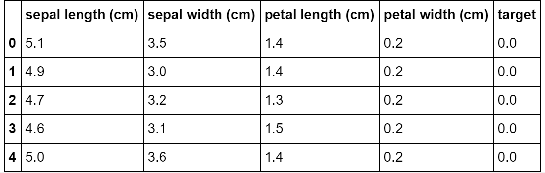
The target column represents the subspecies of iris.

Use train_test_split to Partition the Dataset

The model selection module has several useful functions for splitting the dataset and for hyperparameter tuning. We will be using sklearn.model_selection.train_test_split to randomly partition our dataset into a training set and a testing set.

from sklearn.model_selection import train_test_split

# X captures our feature, y captures the target
y = data['target']
X = data.drop(columns='target')
 
# randomly partition 20% of the data for testing
# setting the seed guarantees that the split can be replicated
X_train, X_test, y_train, y_test = train_test_split(X, y, test_size=0.2, random_state=1)

Feature Selection

How do we know which features we want to use in our model? How do we distinguish relevant predictors from noise? A lot of that comes down to domain knowledge, but this is also a process which can be automated by feature selection techniques. Scikit-learn has an entire module dedicated to that.

We will be using the SelectKbest function to select the most prominent features. By setting k to be the same number of features we have available, we can use these outputs to quantify the importance of each feature. The F-test value for classification will be used as the scoring function.

from sklearn.feature_selection import SelectKBest, f_classif
 
feature_selector = SelectKBest(f_classif, k='all')
feature_selector.fit(X_train, y_train)
 
# get scores for each feature
feature_selector.scores_

The scores suggest that the petal dimensions are much stronger predictors than the sepal dimensions.

These scores are hard to interpret on their own. We need to look at their corresponding p-values to determine the statistical significance of their effect on the target variables.

We can obtain the pvalues from feature_selection.pvalues_

P-value indicates the % of more "extreme" observations if the null hypothesis is true and if we repeat the same experiment many times. The null hypothesis here is that the feature has no effect on the target (i.e. we should not use it as a predictor). Low p-values suggest we should reject our null hypothesis - in other words, reject the claim that the feature has no effect.

In this example, we have very small p-values: 2.65205811e-25, 8.62129460e-13, 1.97685433e-72, 1.15999788e-66. We should keep all 4 variables in the model.

Training the Classifier

Models and algorithms are covered in more detail in subsequent sections. For now, we will gloss over the mechanisms behind these algorithm. Scikit-learn makes it incredibly easy to train a model. All we have to do is instantiate the classifier and call the fit method to train it over the training set.

Here is an example with Logistic Regression.

from sklearn.linear_model import LogisticRegression

# instantiate the model and fit it over the training set
clf = LogisticRegression(random_state=0).fit(X_train, y_train)

# use the model for prediction
new_observation = [1, 1, 2, 3]
 
# get predicted class
clf.predict([new_observation])

# get probability scores for each class
clf.predict_proba([new_observation])
 
# get coefficients (coefficients can be used for interpretability)
clf.coef_

Assessing Performance

After we train our model, we want to assess its performance. This can help us choose between candidate models and communicate model expectations to stakeholders. Scikit-learn's metrics module can help us with this.

First, we use the model to predict labels for our testing set. Then we compare the predicted labels against the true labels to determine the performance.

from sklearn.metrics import accuracy_score, confusion_matrix, classification_report

# predict labels for testing set
y_pred = clf.predict(X_test)

# get accuracy score
accuracy_score(y_test, y_pred)
 
# get confusion matrix
confusion_matrix(y_test, y_pred)
 
# get classification_report
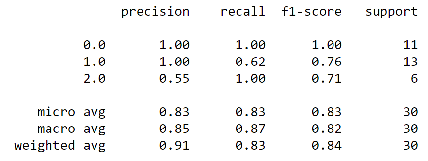
classification_report(y_test, y_pred)

The classification report breaks down the precision, recall and f1-score for each class. There are 3 different ways of calculating the overall f1-score:

The support column indicates the number of observations in each class.

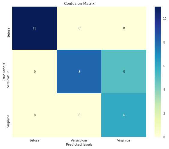
The confusion matrix shows a breakdown of correct and incorrect classifications. The model classifies Setosa very well, but has trouble differentiating between the other two classes.

Here's all of the code we used in one place:

import pandas as pd
import numpy as np
from sklearn.datasets import load_iris
from sklearn.model_selection import train_test_split
from sklearn.feature_selection import SelectKBest, f_classif
from sklearn.linear_model import LogisticRegression
from sklearn.metrics import accuracy_score, confusion_matrix, classification_report

iris = load_iris()

# concatenate feature variables with target
data = np.c_[iris['data'], iris['target']]
data = pd.DataFrame(data=data, columns=iris['feature_names'] + ['target'])

y = data['target']
X = data.drop(columns='target')

# partition training and testing set
X_train, X_test, y_train, y_test = train_test_split(X, y, test_size=0.2, random_state=1)

# get feature selection scores
feature_selector = SelectKBest(f_classif, k=4)
feature_selector.fit(X_train, y_train)
feature_selector.scores_

# instantiate the model and fit it over the training set
clf = LogisticRegression(random_state=0).fit(X_train, y_train)

# predict class for new observation
new_observation = [5, 3, 5.1, 1.5]
clf.predict([new_observation])

# predict labels for testing set
y_pred = clf.predict(X_test)

accuracy_score(y_test, y_pred)
confusion_matrix(y_test, y_pred)
print(classification_report(y_test, y_pred))

Thanks for reading our Scikit-Learn lesson

Here are some additional reading(s) that may be helpful: