Tree-based Models

Tree-based methods can be used for both regression and classification. The idea behind these algorithms is to divide the predictor space into multiple non-overlapping regions and to assign new observations to their respective region. These methods are also known as decision tree methods.

Decision Trees for Regression

After splitting the predictor space into $n$ regions, we calculate a statistic (for instance, the mean) for the response variable in that region. New predictions will be placed into their respective regions and the region's statistic will be used as the prediction.

Let's use the example of house prices to illustrate an example. To keep it simple, we will assume that the optimal regions have already been determined. Jim, the real estate agent, wants to try a tree-based approach for predicting house prices. He is using square footage and age of the home as his predictors.

Jim's decision tree partitions his predictor space as follows:

Region #1: square footage under 250 and age under 10 years

Region #2: square footage under 250 and age over 10 years

Region #3: square footage over 250 and age under 10 years

Region #4: square footage over 250 and age over 10 years

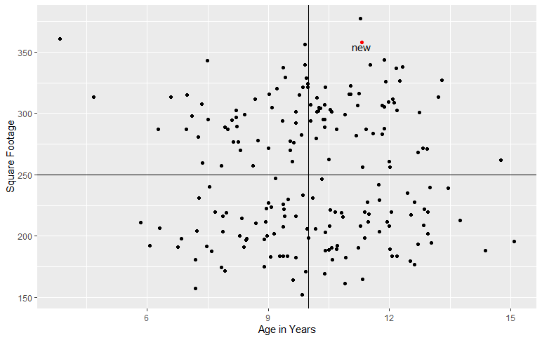
Jim wants to infer the price of a new house (colored red in the plot). This house falls into Region #4. The average price for houses in Region 4 as observed from the training set is $125,000. Thus, Jim's model would predict that this new house would sell for that much.

Decision Trees for Classification

Decision Trees for classification behaves similarly to regression. Assume that Jim decides to use the same predictors (on a different dataset) to predict whether someone will make an offer on a house. The blue observations corresponds to those that made offers while red corresponds to no offer. The algorithm divides the predictor space into $n$ regions and each region is mapped to a class.

Region #1: age under 5 years

Region #2: age over 5 years and square footage over 250

Region #3: age over 5 years and square footage under 250

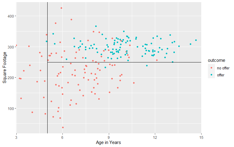
Let's assume that the algorithm also tells us that Regions 2 and 3 are mapped to "offer", while Region 1 is mapped to "no offer". With this information, we can predict which class subsequent observations will fall under.

More Complex Tree-Based Methods

We can ensemble (combine) multiple decision trees to form more complex models. Tree-based ensembling algorithms are divided into:

Bagging (also known as bootstrap aggregation): smaller subsets of the data is created via random sampling with replacement. A decision tree is trained over each subset. The results from each decision tree is averaged to produce the final output.

Boosting: unlike Bagging where each decision tree is trained independently, each learner in the Boosting algorithm learns sequentially from previous learners.

Stacking: several models are trained in parallel. Another model is trained to determine the output based on the predictions of each ensembled model. This ensemble technique is not as common for tree-based models.

Bagging Example: Random Forest

Random Forest is a popular Machine Learning algorithm which ensembles decision trees using bagging. In addition to randomly sampling the training data for each tree, Random Forests also randomly sample the features used for each tree.

Boosting Example: AdaBoost with Decision Trees

AdaBoost, which is short for adaptive boosting, ensembles decision trees in an iterative process: we start with one decision tree trained over the dataset, but at each iterative step, we reweigh the dataset to give more emphasis to the misclassifications and retrain the decision tree over this reweighted dataset.

« Previous: Logistic Regression Tutorials Next: Support Vector Machines »