Data Cleaning

Data cleaning is the process of correcting or removing inaccurate records from a dataset. We can also "clean" the data using normalization, the process of reducing data to a canonical form. These steps are usually performed prior to model development, but also required when inferencing.

We will illustrate data cleaning using a messy dataset.

Getting Started

Once again, we will use the Pandas library to read data into a DataFrame. Run pip install pandas==0.24.2 to install the same version that we are using.

We will use the 2018 Kaggle ML & DS Survey dataset for our example. Kaggle is an online community that brings AI practitioners together to tackle Data Science problems and to share datasets. Kaggle datasets can be downloaded programmatically using their API, but for now, we will manually download the data.

Understanding the Data

Common sense, prior knowledge and context helps us recognize inaccurate records and biases contained in the dataset. Kaggle conducted this survey with its members to get a more "comprehensive view of the state of data science and machine learning" in 2018. We should recognize that Kaggle respondents may not be representative of the entire Data Science community and communicate these biases alongside our findings.

Loading the Data

For this exercise, we will work exclusively with multipleChoiceResponses.csv, which aggregates the respondents' answers to multiple choice questions. This dataset is a good representation of data found in the real world: biased and messy with potentially inaccurate records.

With the way that this data is formatted, we have to remove the first row for each survey question to be its own column name. We can use iloc to filter the dataframe based on its row and column indices.

import pandas as pd
data = pd.read_csv('multipleChoiceResponses.csv')
data = data.iloc[1:, :]

This loads the dataset into the data object. We can use the .head() method to take a peek at what it looks like (only the first eight columns and first five rows are displayed).

data.head()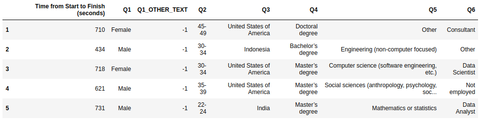

Removing Potentially Erroneous Inputs

Erroneous inputs can occur if someone deliberately lied on the survey, misunderstood the question or selected the wrong answer by mistake. We need to identify and remove these responses. The distribution of the Time from Start to Finish (seconds) shows that some of these surveys were answered very quickly.

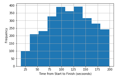
For a survey with 19 questions, we can assume that any response provided in under a minute is unlikely to be accurate. This threshold was arbitrarily selected. We could have determined it by measuring the amount of time required to read the questions or we can use a more mathematical approach to find breaks within the distribution.

This exclude records not satisfying data['Time from Start to Finish (seconds)'] >= 60.

data = data[data['Time from Start to Finish (seconds)'].astype(int) >= 60]

We can also check and correct logical inconsistencies. An example of a logical inconsistency could be someone who is employed, but reporting an income of zero. We can "fix" these responses by mapping all zero incomes to an unemployed status.

It is also worthwhile to de-duplicate the data. If someone answers the survey multiple times, we probably don't want to double count their response.

Extreme Observations

Together, erroneous inputs and extreme observations makes up outliers -- data points that differ significantly from the other observations. Someone who finishes the survey in under 5 seconds most likely scripted the response (erroneous input), but a super speed reader might be able to complete the survey in 60 seconds while providing accurate information.

There are several definitions used to identify outliers. One of the most straightforward definitions suggests that any data points more than 1.5 interquartile ranges (difference between the first and third quartile) below the first quartile or above the third quartile are considered outliers. We can also use anomaly detection methods to determine outliers based on a larger feature space.

Normalizing Survey Responses

We might want to normalize certain answers to reduce the dimensionality of the data and make it easier to interpret the results.

For instance, we might recognize that some of the possible occupations from Question 6, designation or title, are very similar. If we wanted to use this response as a predictor for education level, we might combine or normalize occupation based on their education requirements.

We can do this by defining a mapping and using apply to specify the function used to create this new normalized column for Q6.

job_mapping = {
  'Salesperson': 'business role',
  'Marketing Analyst': 'business role',
  'Business Analyst': 'business role',
  'Software Engineer': 'engineering',
  'Developer Advocate': 'engineering',
  'Data Engineer': 'engineering',
  'DBA/Database Engineer': 'engineering',
  'Data Scientist': 'other data roles',
  'Data Analyst': 'other data roles',
  'Statistician': 'other data roles'
}

data['normalized_Q6'] = data['Q6'].apply(lambda x: job_mapping[x] if x in job_mapping.keys() else 'other')

Try it out yourself!