Sentiment Analysis with Wine Reviews

Photo by Kelsey Knight on Unsplash
Note: this was an older guide we wrote in 2018. At the time of writing, these methods were considered state of the art for Natural Language Processing. A lot has changed since then, but using a Recurrent Neural Network with GRU units trained on GloVe embeddings should still be able to yield a useful classifier.
We will be using this Kaggle data set which contains wine reviews, the rating of the wine (measured in points) and other relevant information scraped from WineEnthusiasts. The data set contains two files scraped on separate days. Let's use winemag-data_first150k.csv as the training set and winemag-data-130k-v2.csv (scrapes from a later date) as the testing est.
Here is the repository for the code.
Objective: Train a Machine Learning model which predicts Wine Quality based on Text Review
WineEnthusiasts use a points scale ranging from 1 to 100 to rate their wines (1 being the worst, 100 being the best). Unfortunately, the website only shares positive reviews, which is why the range of the scores in the data set only range from 80 to 100.
This means that our data set is not representative of the problem we are trying to tackle. Any models built using this data would only be applicable to well received wines.
Gather some domain knowledge
Before we start with our analysis, we should try to gather some domain knowledge. After exploring the website and reading some other wine related resources, I found a nifty classification system based on the points system.
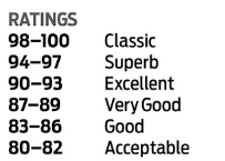
To an end user (i.e. wine shopper), the points are only as important as the information they convey. If we frame this as a classification problem with the above breakdown, we can still convey wine quality while reducing the dimensionality of the problem.
As such, this becomes a Sentiment Analysis problem where we will use the text reviews to predict whether a wine is Classic, Superb, Excellent, Very Good, Good or Acceptable.
Exploratory Data Analysis
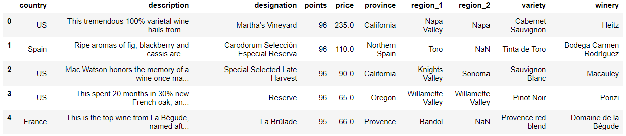
The next step is getting to know our data a little better. This can give us important insights to tackle the problem better. In addition to the review and rating, there are other relevant information such as the wine price, variety (grape type) and location the wine was produced.
To train a more comprehensive model, we can also include these features as predictors to predict the quality. To combine text descriptions with other predictive features, we can either create an ensemble model (with the text classifier being one of them) or a hierarchical model where the results from the text classifier will be used as a predictive variable.
In this guide, we will only be exploring the relationship between the text review and wine score.
Examining Data Integrity at a High Level
There are no missing entries from the points and description column. As we have noticed before, the wine points are skewed to the higher end of the scale. From personal experience, the prices are also on the higher end of the scale.
import pandas as pd

data = pd.read_csv("winemag-data_first150k.csv", index_col = False)
data.describe()
data.info()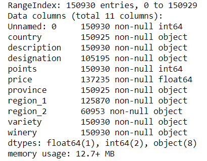
Examining the Textual Data
The reviews look very “clean”. There doesn’t seem to be any grammatical nor spelling errors and all reviews are written in very concise language. Here is a sample review:
This tremendous 100% varietal wine hails from Oakville and was aged over three years in oak. Juicy red-cherry fruit and a compelling hint of caramel greet the palate, framed by elegant, fine tannins and a subtle minty tone in the background. Balanced and rewarding from start to finish, it has years ahead of it to develop further nuance. Enjoy 2022–2030.
Some of the reviews require wine knowledge to fully understand. In the above example, tannin is a textual element that makes wine taste dry. We can take a look at how frequently certain vocabulary terms appear.
import seaborn as sns
import matplotlib.pyplot as plt
from nltk.tokenize.treebank import TreebankWordDetokenizer
from nltk.corpus import stopwords
from nltk import word_tokenize

# set seaborn style
sns.set(style="whitegrid")

stopwords = set(stopwords.words('english'))

# Detokenizer combines tokenized elements
detokenizer = TreebankWordDetokenizer()

def clean_description(desc):
  desc = word_tokenize(desc.lower())
  desc = [token for token in desc if token not in stopwords and token.isalpha()]
  return detokenizer.detokenize(desc)

data["cleaned_description"] = data["description"].apply(clean_description)

word_occurrence = data["cleaned_description"].str.split(expand=True).stack().value_counts()
total_words = sum(word_occurrence)

# plot most common words
top_words = word_occurrence[:30]/total_words

ax = sns.barplot(x = top_words.values, y = top_words.index)
ax.set_title("% Occurrence of Most Frequent Words")

plt.show()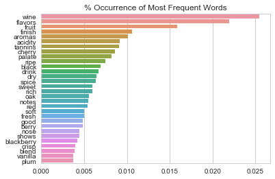
Preparing for Classification
We can create a new column in our DataFrame which will use the points break down outlined above to create the target class. Unfortunately, our classes are not very balanced.
| Number of Reviews | |
|---|---|
| Class 0: Acceptable (80-83 points) | 6441 |
| Class 1: Good (83-86 points) | 44740 |
| Class 2: Very Good (87-89 points) | 51539 |
| Class 3: Excellent (90-93 points) | 41767 |
| Class 4: Superb (94-97 points) | 0 |
| Class 5: Classic (98-100 points) | 6443 |
There are no reviews in Class 4 (94–97 points — Superb) and most of the reviews are concentrated in Classes 1,2 and 3. Unbalanced classes are problematic, but can be addressed by sampling the larger classes or setting class weights. The total absence of one class, however, is much more concerning.
Let's combine Classes 4 and 5 into a new class Very Good/Superb.
Should the Textual Data be cleaned?
We also have the option of cleaning/normalizing our wine reviews. The biggest factor affecting this decision is the type of learning algorithm we want to use. If we choose to embed each review as its own vector and pass the input into an one-to-one classifier, then we should spend a great deal more time normalizing the text. On the other hand, processing the text sequentially as a representation of many vectors makes normalizing less important.
Processing the text sequentially (where typically each word is represented by its own vector and word relationships are learned) also helps address word-sense disambiguation (the same word possessing multiple meanings) and identify synonyms.
We can train a Recurrent Neural Network to learn each review token by token where each token is mapped to its own vector. This way, the learning algorithm will also learn the ordering of each word and how that can affect the sentiment of the review.
We have the option of using pre-trained embeddings, train our own or fine tune pre-trained embeddings with this corpus. To make things easier, let's use pre-trained GloVe vectors.
Several pre-trained GloVe word vectors can be downloaded here.
Let's use the Common Crawl with 840B tokens as it contains the largest vocabulary and is also case sensitive. Each word vector from glove.840B.300d has 300 coordinates.
Before loading the pre-trained embeddings, we should define some fixed parameters:
num_classes = 5  # this represents the number of classes
embedding_dim = 300  # dimension of the word vectors
epochs = 5  # number of forward and backward passes through all of the training examples
batch_size = 128  # number of training examples in each pass
max_len = 100  # max length (in words) a text review can have
class_weights = {0: 7, 1: 1, 2: 1, 3: 1, 4: 7}
For the maximum length, any descriptions with more than 100 words will be truncated. Any descriptions with less than 100 words will be padded to meet this length. The class weights are used to give more emphasis on the minority classes. Classes with higher weights attached to them (class 0 and class 4) will have a higher impact on the learning algorithm. Each instance of class 0 is treated as 7 instances.
Let's start training the classifier. First, loading the required libraries.
import pandas as pd
import numpy as np

from keras.models import Model, load_model
from keras.layers import Dense, Embedding, Input, Activation, GRU, Bidirectional, Dropout, GlobalMaxPooling1D
from keras.preprocessing.text import Tokenizer
from keras.preprocessing.sequence import pad_sequences
from keras.callbacks import EarlyStopping, ModelCheckpoint, Callback
from sklearn.model_selection import train_test_split
We need to one-hot encode the target class.
def onehot(arr, num_class):
  return np.eye(num_class)[np.array(arr.astype(int)).reshape(-1)]

y = onehot(data["rating"], num_classes)
Even though we already have a designated test set, it can still be a good idea to divide the training set into training and validation for the purpose of parameter tuning.
X_train, X_val, y_train, y_val = train_test_split(data["description"], y, test_size = 0.05)Tokenizing Inputs and Preparing the Embedding Matrix
We will be using Keras’s text_to_sequences method to preserve the word sequence of the text. Each word will be mapped to its vector from the pre-trained word vectors. Any descriptions under 100 (max_len) words will be padded and any descriptions over 100 (max_len) words will be truncated so that the input is the same length.
Words found in the text that do not appear in the vocabulary of the pre-trained word vectors are initialized to the zero vector (can you think of better ways to initialize out of vocabulary words?)
# Prepare embeddings
# Embedding file not contained in repo. Download from https://nlp.stanford.edu/projects/glove/
# Here, we are using glove.840B.300d.zip

embeddings_index = {}

# Read pre-trained word vectors and populate to dictionary
f = open("glove.840B.300d.txt", encoding = "utf8")

for line in f:
  values = line.split()
  word = ''.join(values[:-embedding_dim])
  coefs = np.asarray(values[-embedding_dim:], dtype='float32')
  embeddings_index[word] = coefs
f.close()

# train tokenizer
tokenizer = Tokenizer(num_words = None)
tokenizer.fit_on_texts(X_train)

# fit tokenizer
sequences_train = tokenizer.texts_to_sequences(X_train)

# Padding any short sequences with 0s
X_train = pad_sequences(sequences_train, maxlen=max_len)

sequences_val = tokenizer.texts_to_sequences(X_val)
X_val = pad_sequences(sequences_val, maxlen = max_len)

word_index = tokenizer.word_index

# create embedding layer
# We can designate "Out of Vocabulary" word vectors here
# In this case, they are initialized to zero vector
embedding_matrix = np.zeros((len(word_index) + 1, embedding_dim))

for word, i in word_index.items():
  embedding_vector = embeddings_index.get(word)
  if embedding_vector is not None:
    embedding_matrix[i] = embedding_vector
Training the Classifier
Since the text descriptions are generally short, we should use GRU units as opposed to LSTM units. With shorter descriptions, we have less need for a memory unit and can benefit from GRU’s more efficient learning algorithm.
We will also be utilizing early stopping, which (in this case) uses validation accuracy to determine whether we should continue training the network. When validation accuracy continuously drops over several epochs, early stopping will kick in and end the training process. It will also save the optimal weights as a “checkpoint” (in this case as model.h5) and rewrite the weights if accuracy improves. With early stopping, we can let the network train for many epochs without worrying too much about overfitting.
The patience parameter is a threshold used to determine if/when to prematurely end training. Patience = 3 indicates that an early stop will be initiated if there are no improvements to validation loss after 3 epochs.
embedding_layer = Embedding(len(word_index) + 1, embedding_dim, weights = [embedding_matrix], input_length = max_len, trainable = False)
input= Input(shape=(max_len, ), dtype = 'int32')
embedded_sequences = embedding_layer(input)
x = Bidirectional(GRU(50, return_sequences=True))(embedded_sequences)
x = GlobalMaxPooling1D()(x)
x = Dense(50, activation = 'relu')(x)
x = Dropout(0.1)(x)
output = Dense(num_classes, activation='softmax')(x)
model = Model(inputs=input, outputs=output)
model.compile(loss="categorical_crossentropy", optimizer='adam', metrics=['accuracy'])

checkpoint = ModelCheckpoint("model.h5", monitor='val_loss', verbose=1, save_best_only=True, mode='min')
early = EarlyStopping(monitor='val_loss', mode='min', patience=3)
callback = [checkpoint, early]

model.fit(X_train, y_train, batch_size=batch_size, epochs=epochs, validation_data=(X_val, y_val), callbacks=callback, class_weight = class_weights)
The structure of the Recurrent Neural Network is quite simple. The network has one bidirectional GRU layer with 50 units followed by a pooling, dense and dropout layer. Bidirectional means that the network will learn the text sequences in their original order as well as the reverse order in which the words appear.
The classifier uses the correctness of the predictions to learn. It does not differentiate between incorrect predictions the way a human might. To a human, predicting a Class 0 as a Class 4 will be worse than predicting a Class 0 to be a Class 1. To the network, it makes no difference. For future implementations, it might be worthwhile to devise a metric which reflects this relationship.
It’s time to assess our model — let’s bring out the test set!
from sklearn.metrics import accuracy_score

test = pd.read_csv("winemag-data-130k-v2.csv", index_col = False)
test["rating"] = test["points"].apply(points_to_class)

sequences_test = tokenizer.texts_to_sequences(test["description"])
X_test = pad_sequences(sequences_test, maxlen=max_len)

# Predictions
pred_test = model.predict(X_test)
pred_test = [np.argmax(x) for x in pred_test]

# Actual
true_test = onehot(test["rating"], num_class)
true_test = [np.argmax(x) for x in true_test]

# Find accuracies
accuracy = accuracy_score(true_test, pred_test)
Accuracy over Test Set: 64%
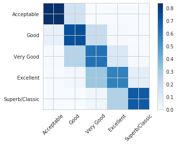
Let’s take a look at the confusion matrix. In this matrix, the values are measured as percentages to reflect the unbalanced nature of our data.
from sklearn.metrics import confusion_matrix

cm = confusion_matrix(true_test, pred_test)
cm = cm.astype('float') / cm.sum(axis=1)[:, np.newaxis]

plt.imshow(cm, interpolation='nearest', cmap=plt.cm.Blues)

class_name = ["Acceptable", "Good", "Very Good", "Excellent", "Superb/Classic"]
plt.colorbar()
tick_marks = np.arange(len(class_name))
plt.xticks(tick_marks, class_name, rotation=45)
plt.yticks(tick_marks, class_name)

plt.show()